
Menu:
Home
HA 2000:6
A SYNTHESIS OF THEORIES ON THE LONG-RUN PHILLIPS CURVES
byFritz C. Holte
|
Menu: Home |
HA 2000:6
A SYNTHESIS OF THEORIES ON THE LONG-RUN PHILLIPS CURVESbyFritz C. Holte |
I shall now present a price theory which is probably accepted by a majority of the economists today. I call it "the price theory of the 1990s" even though it was developed earlier.
The long-run Phillips curve is a curve which shows the combinations of unemployment and price change which keep the price change constant. According to the price theory of the 1990s unemployment is the same in all those combinations, as illustrated by Figure I.1.
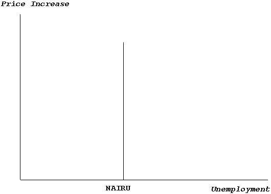 |
| Figure I.1 |
| The long-run Phillips curve used in the theory of the 1990s |
Another curve is called the short-run Phillips curve. It is used when economists describe what happens in the short run.
The unemployment rate which keeps price change constant is usually called either NAIRU (Non-Accelerating Rate of Unemployment) or "the equilibrium unemployment".
The factors which determine the value of NAIRU belong to what economists call "the supply side of the product market" 1. Among them are the amount of mismatch and wage-setting.
The factors which determines NAIRU change over time. Therefore NAIRU changes over time.
Suppose for a moment that unemployment by means of political measures or for some other reason remains constant at a level which is lower than NAIRU. Then prices will accelerate, i.e. "the price increase" will increase.
Suppose next that the unemployment remains constant at a level which is higher than NAIRU. Here prices will decelerate, i.e. "the price change" will decrease.
By an economic shock we mean something which rapidly leads to a considerable change in the conditions for economic behaviour. We can get economic shocks both on the demand side of the product market and on its supply side.
Economic shocks usually make unemployment different from NAIRU. When such differences occur, they activate economic mechanisms which make unemployment approach NAIRU.2 If there are no new shocks for a sufficiently long time, these mechanisms will make unemployment equal to NAIRU.
In the late l950s and throughout most of the 1960s it was common to use a Phillips curve which falls as one moves to the right in a diagram where we measure unemployment and price increase along the axes (cf. Figure I.2). In that period economists did not distinguish between Phillips curves in the long and short runs. Therefore it seems reasonable to regard the curve in Figure I.2 as both a long-run and a short-run Phillips curve.
In the 1950s it was common to reason as follows: The authorities want both low unemployment and low inflation. The Phillips curve can be seen as a menu for politicians. Using this menu they can choose low employment, but then they must accept that prices increase rapidly. Or they can choose a low price-increase. But the slower the prices increase they choose, the more unemployment they must accept.
The theory expressed by Figure I.2 will hereafter be called the price theory of the 1950s.
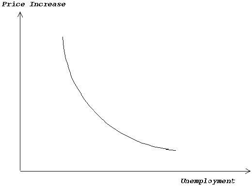 |
| Figure I.2 |
| The Phillips curve used in the theory of the 1050s |
These two theories are not used in the price theory of the 1990s:
Theory no. 1 is probably fairly indisputable. Several factors may contribute to make theory no. 2 likely. Here are two of them:
If a producer reduces the prices of his products, other producers in the same industry may regard this as an attempt to increase the producer's share of the market. Such interpretations can start a "price war" which will not be advantageous to any producer, and which therefore none of them wants. To refrain from increasing the price of a product as much as the general price level increases, will not be regarded as an invitation to a price war.
Many producers have stocks of goods they have manufactured, but not yet sold. Reducing the prices of these goods can mean that the money gained by selling them would be less than what it has cost to produce them. Reduced prices will therefore lead to registered losses, and some producers seek to avoid registered losses. This affect their price-setting, although it can be argued that it is not rational to let the price policy be influenced by so-called sunken costs.
A greatly simplified example will be used to exemplify an important point.
I shall assume that:
Let us assume that prices rose by 7% from 1994 to 1995.
Towards the end of 1995 the price-leader in A shall set its prices for 1996. At that time it is difficult to sell A-products. Therefore this price-leader believes that it will be advantageous if his products become somewhat cheaper compared to the price-level. He knows that prices rose by 7% from 1994 to 1995, and he expects B-prices to rise at least that much from 1995 to 1996. On the basis of this, the price-leader in A increases his prices by 5%. The other producers in A do the same.
For the B industry the prospects look good. As a result, the price-leader in B believes that will be advantageous if his prices increase somewhat faster than they did the previous year. So he raises his prices by 8% from 1995 to 1996, and the other B-producers do the same.
According to what is assumed above, A-prices will increase by 5%, whereas B prices will increase by 8%. The price level, which is the average of A-prices and B-prices, will therefore rise by 6.5%. This means that the price-increase will be 0.5% lower than it was from 1994 to 1995.
We shall now turn to another situation. Let us assume that the price level remains unchanged from 1994 to 1995, but that all other conditions, including unemployment and conditions in the product markets, are the same as assumed above. The combination of a stable price level and sales difficulties for A-products, activates a disinclination to reduce prices within A. Because of this activation A-prices will be the same in 1996 as they were in 1995, despite the marketing difficulties for the A-industry. For B, on the other hand, marketing possibilities look so good that the B-firms raise their prices by 1%. No change in the A-prices and 1% increase in the B-prices means that the price-level increases by 0.5% from 1995 to 1996.
Let us compare the two situations. Even though the unemployment is the same in both situations, the price level increase in the second case, but decrease in the first one. The reason for this difference is that the disinclination towards price-reduction is activated in the second situation but not in the first.
This example sheds light on two points. One is that when the increase in the price-level is low, a disinclination to reduce prices is activated. The other is that this disinclination influences the development of the price-level.
I have discussed a highly simplified case. But the disinclination to reduce prices influence the development of the prices also in countries where there are more than two industries, and where prices are set in other ways than in my example.
In what follows I shall present a theory which can be called the synthesis of the theories of the 1950s and the 1990s on the long-run Phillips curve. Figure I.3 will be used in this presentation.
By inflation, as usually is done, we mean the increase in the price level.
Unemployment less than H. If the unemployment rate is lower than a certain limit, which in Figure I.3 is called H, the inflation increase. (Cf. what happens according to the price theory of the 1990s when unemployment is less than NAIRU.)
Unemployment higher than R. If the unemployment rate is higher than another limit, which is called R in the figure, the inflation decrease. This implies that sooner or later the price level changes from rising to falling, and after that falls faster and faster.
If the unemployment rate is larger than H but less than R, we will say it is in the menu interval.
What happens if unemployment is constant and is in the menu interval? Until otherwise stated, we shall assume that the authorities follow a policy that make sure that unemployment does not change. Therefore, if conditions change, the change is only in the rate of inflation. Or, to put this in terms of the diagram: if we move in Figure I.3, the movement is along a vertical line.
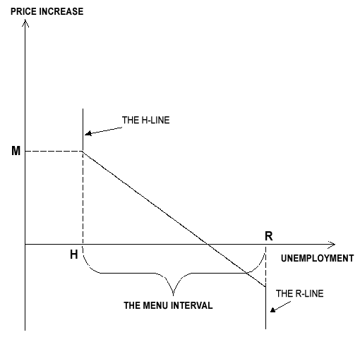 |
| Figure I.3 |
| The three-part long-run Phillips curve |
I shall assume that we start in a situation where the unemployment is in the menu interval, and where the inflation is so high that no producer can be interested in reducing its prices. In Figure I.3 this situation will be represented by a point which lies above thee long-run Phillips curve.
If a producer wants its prices to become lower compared to other prices, this can be achieved by increasing his prices slower than the price level. (Cf. the first part of the simplified example.) Under such conditions, no disinclination to reduce prices will be activated.
I shall also assume that as long as no disinclination to reduce prices is activated, inflation decreases. (Cf. again the first part of the simplified example.)
After inflation has decreased for some time it will have become so low that in some firms a disinclination to reduce prices is activated. That disinclination acts as a brake on the further reduction of the inflation. At first that brake is not strong enough to stop the reduction, but only reduces its speed.
As long as inflation decreases, "the disinclination" is activated in more and more firms, and "the brake" therefore becomes stronger and stronger. Sooner or later inflation has become so low that we get the following situation: the activated disinclination to reduce prices is exactly strong enough to match the market forces which push towards reduced inflation. This implies that inflation remains constant.
If inflation for some reason becomes lower than in this situation, we get conditions where the disinclination to cut prices is stronger than the market forces that push towards lower inflation. If that happens, inflation increases. (Cf. the last part of the simplified example.)
With reference to Figure I.3, we can describe what happens as follows: Moving downwards along a vertical line in the diagram we reach one, and only one, point on the long-run Phillips curve. (Remember that the long-run Phillips curve consists of those points, and only those points, which each represent a combination of unemployment and inflation that makes inflation constant.)
What happens if unemployment changes, but still remains within the menu interval? The more difficult it is for a firm to sell its products, the stronger are the market forces, which pull in the direction of decreasing inflation. This means that the larger the marketing difficulties are, the more disinclination to cut prices must be activated before the inflation is stabilized. Therefore, the larger the marketing difficulties are, the lower will be the rate of inflation which makes inflation stable.
Unemployment can serve as an indicator of the marketing difficulties. The larger the marketing difficulties are, the higher unemployment there will be. From this and from the discussion in the preceding paragraph we can conclude:
In line with this conclusion, the menu in Figure I.3 is drawn as a curve which falls as we move towards the right in the diagram. In order to simplify things, the curve is drawn as a straight line. That is probably unlikely, but we need not be concerned with that here.
Unemployment equals H. Suppose that unemployment equals H, i.e. it lies at the lower limit of the menu interval.
We shall assume that we start in a situation where the price-level is rising so fast that no firm can be interested in reducing its prices. This means that no disinclination to reduce prices is activated. We shall also assume that in this situation the forces which pull in the direction of lower inflation are exactly as strong as those pulling in the opposite direction. This means that the rate of inflation remains constant.
Let us now turn to a situation where inflation is lower than in the situation discussed above. If it is low enough we have a situation where it will be rational for one or more firms to reduce their prices. This activates the disinclination to reduce prices. As a result of that, the forces pulling towards a decrease in the price level are weaker than the forces pulling towards an increase. Consequently, inflation increases.
What is said above can be summed up in this way: If unemployment is equal to H, the inflation remains constant if and only if, it is above a certain level. In Figure I.3 that level is called M. The conclusion that the inflation is constant if, and only if, it is above M, is expressed by letting a line called the H-line be part of the Phillips curve.
Unemployment equals R. By reasoning in the same way as above, we can also conclude: If unemployment equals R, the inflation remains constant if, and only if, it lies under a certain level. In Figure I.3 this is expressed by letting the R-line be part of the Phillips curve.
The long-run Phillips curve in Figure I.3 has two parts that are vertical lines, one connected to unemployment H, the other to unemployment R. These parts have the form we should expect from the theory of the 1990s. According to that theory the long-run Phillips curve is a vertical line.
The curve in Figure I.3 also has one part which falls as we move to the right of the diagram. This part has the form we should expect from the theory of the 1950s. According to that theory the Phillips curve falls as we move to the right.
On the basis of what was said above, we can regard the curve in Figure I.3 as a synthesis of the long-run Phillips curves from the 1990s and the 1950s.
If my intention had been to present a comprehensive description of factors which influence the prices, I would have put forth a theory that is different from the one presented above. The conditions in the labour market would have been among the subjects I would have taken up.
However, my aim has not been to give as comprehensive a description as possible. I have instead focused on only some conditions which influence the price-development. My view is that these conditions provide sufficient grounds for assuming that the long-run Phillips curve consists of three parts.
There are several other conceivable explanations of what we can call the three-part long-run Phillips curve. In one of them we could use the following two theories:
By using these theories in the same way I used theories no.1 and no. 2 in the simplified example, we can argue for the three-part long-run Phillips Curve.
It would have been appropriate to end this article with results from econometric tests of the hypothesis that the long-run Phillips curve consists of three parts. But as far as I know, such tests are not available. Attempts to estimate long-run Phillips curves have in recent years usually (always?) been based on the theory of the 1990s. In other words, the possibility of a three-part long-run Phillips curve has been "assumed away" before data on unemployment and price increases have been analyzed.
Some economists argue as follows:
Here are my comments:
Under the conditions sketched above I must use economic theory - and not empirical evidence - when I am going to choose between the vertical and the three-part long-run Phillips curves. For reasons presented in this article I choose the three-part Phillips curve. One of these reasons is that I regard the argument for the vertical Phillips curve as weak because it is bases only on macroeconomics. It seems reasonable to me to believe that differences between industries have consequences for the form of the long-run Phillips curve.
1 Economists distinguish between factors on the demand side and factors on the supply side of the product market. Roughly speaking the factors on the demand side are the ones which influence saving, investments and demand policy. Conditions in the labour market and the amount of competition among the producers are important factors on the supply side of the product market.
2 According to mainstream economic theory one such mechanism is the so-called real balance effect, which is as follows: High unemployment reduces the price level. Decreasing price level increase the real value of people's financial assets, and therefore makes them richer. Because they become richer, they increase their demand for products. Increased demand for products increases the number of jobs. More jobs means less unemployment.
There is also at least one theory which says that high unemployment will, as a result of low interest rates, increase the demand for products, and therefore reduce unemployment.